How to Filter Dynamic Outcomes
While the SAS Flex Call Log allows you to filter calls based on Static Outcomes that you create within your Settings, Dynamic Outcomes are unable to be filtered within your Call Log and Reports. This is because Dynamic Outcomes are created when the call is saved based on what is selected in the script.
For example, if you have a Specific Person path that includes 1 employee, you may only need 1 Outcome: "Calling for Tony Stark." Whereas if you have a Specific Person path with 20 employees, you can avoid creating 20 separate Outcomes by using a Dynamic Outcome with a collector in the Outcome label. When the call is saved, the Outcome label will populate based on which option or path was selected. Depending on how the agent navigated through the call, the label will vary:

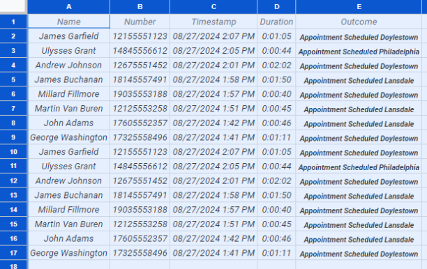
In this tutorial we will show you how to manually filter Dynamic Outcomes using Google Sheets.
1
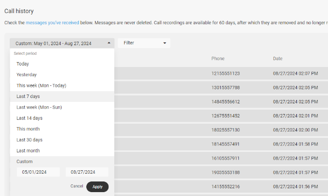
From your call log, adjust your date range to display the calls you want to filter and click Apply.

2
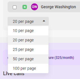
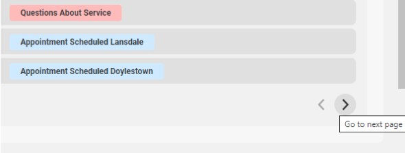
If needed, increase the number of records displayed per page to the maximum.

3
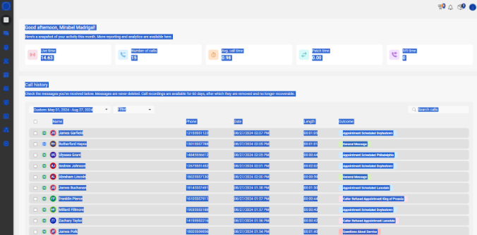
Then, Ctrl+A to highlight everything, and Ctrl+C to copy.

4
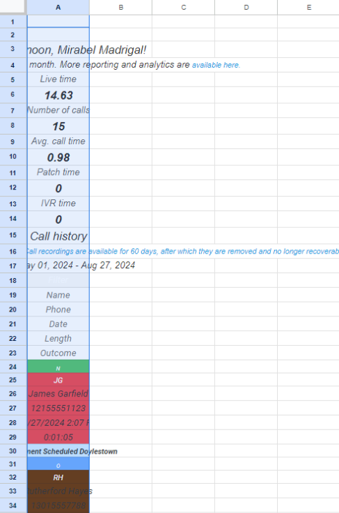
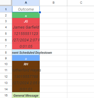
Open Google Sheets, and Ctrl+V to paste the data onto a worksheet. It will look similar to this:

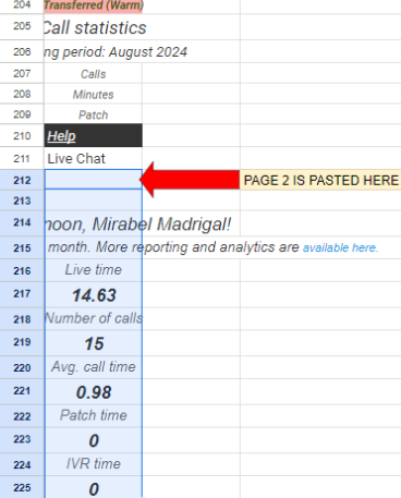
Depending on how many Call Log pages you are copying, you may be able to do all of this on the same sheet - moving forward in the call log to copy each page, and pasting it below the previous data.


5
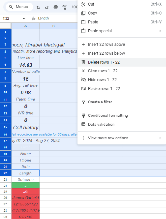
Now that all Call Log data has been pasted, highlight all rows above Outcome, and delete them.

Cell A1 in your top row will now be "Outcome."

6
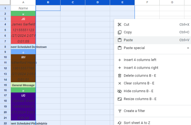
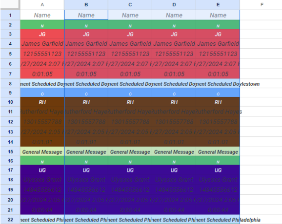
Change “Outcome” to “Name.” Click to highlight the entire column, then paste it 4 times to the right.


7
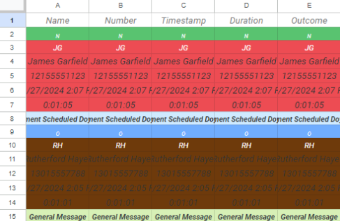
Change the names listed in B1, C1, D1, and E1 to “Number,” “Timestamp,” “Duration,” and “Outcome” respectively.

8
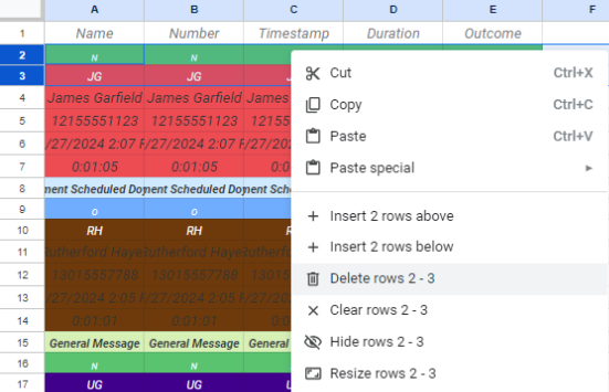
Delete rows 2 and 3.

9
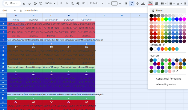
Now, Ctrl+A to highlight the sheet and reset the fill color.

10
In the next few steps, you’ll be removing individual cells from columns B through E to align the data with the corresponding header.
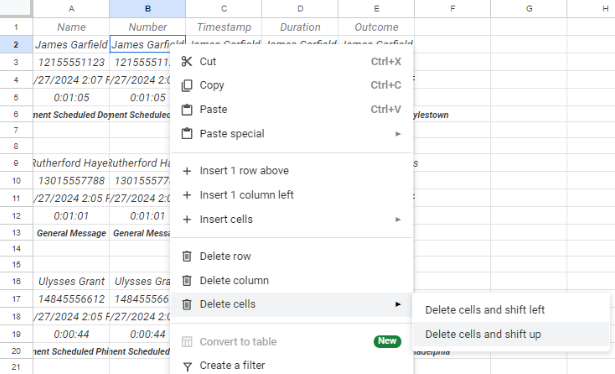
Begin by deleting cell B2 and shifting cells up.

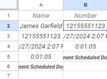
Number will now be in cell B2.

11
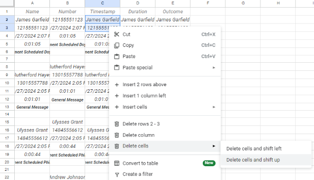
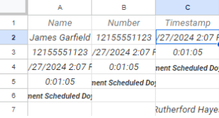
Delete cells C2 and C3, and shift cells up.

Timestamp will now be in cell C2.

12
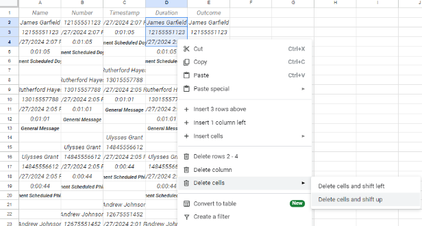
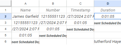
Delete cells D2, D3, and D4, and shift cells up.

Duration will now be in cell D2.

13
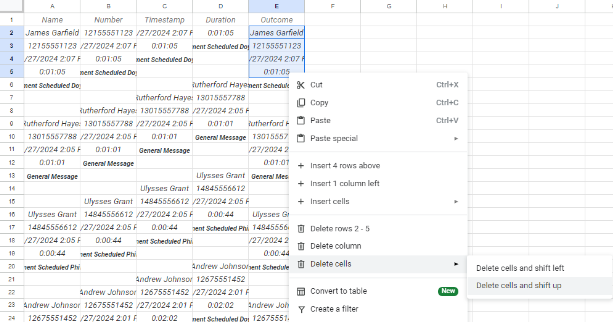
Delete cells E2, E3, E4, and E5, and shift cells up.

Outcome will now be in cell E2.

14
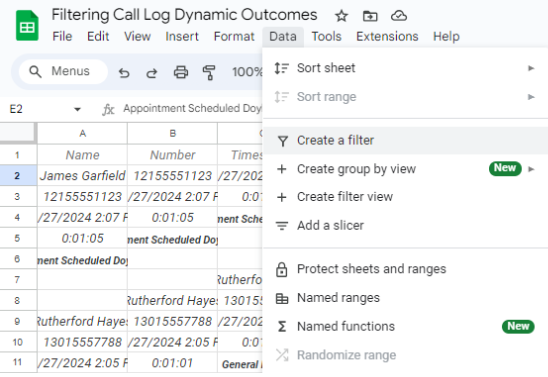
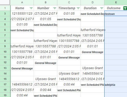
Under Data, click Create a filter.

15
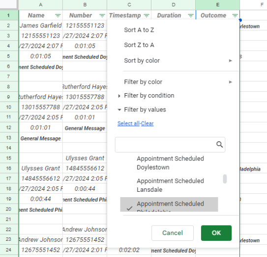
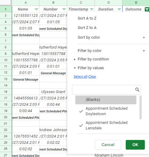
Filter column E to deselect the Outcomes that you need to view. Then, click OK.

16
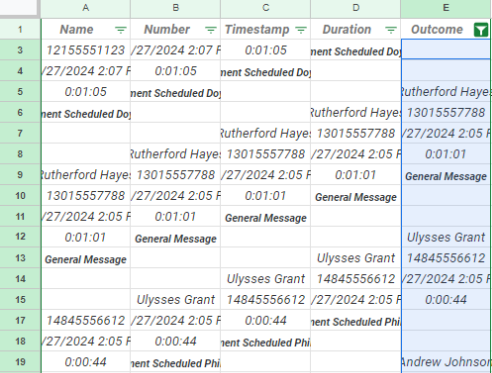
Once filtered, highlight all filtered cells in column E except the header in E1. Do not highlight the entire column.

17
Click Delete. Leave column E filtered. It will be blank except for the header and any data that has spilled over from the previous column.

18
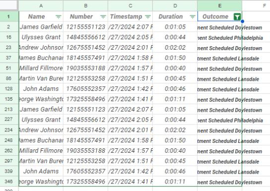
Next, filter again to select the Outcomes you need to view, and deselect Blanks. Click OK.

Only the Outcomes you need will remain.

19
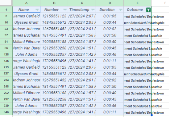
At this point, highlight only the cells containing the remaining data.
Do not use Ctrl+A.
Then, Ctrl+C to copy.

20
Open a new worksheet, Ctrl+V to paste, and adjust your column width so that all data is visible. Format as needed.
